Supervised Machine Learning: Regression and Classification

Supervised Machine Learning: Regression and Classification

Machine learning is a field of study that gives computers the ability to learn without being explicitly programmed.

Supervised vs. Unsupervised Machine Learning

Supervised Learning

Algorithms that know x → y or do input to output mappings are Supervised Learning algorithms. This means that you give your learning algorithms examples to learn from, giving the inputs (x) and telling the desired output (y).

Regression and Classification algorithms use supervised learning.

Regression models are used to predict continuous values, such as the price of a house or the weight of a person. These models are trained using labeled data, where the output or label is a continuous value. The goal of a regression model is to learn a mapping from inputs (also known as features) to the continuous output. Common examples of regression models include linear regression and polynomial regression.

Classification models are used to predict categorical values, such as whether an email is spam or not, or which type of fruit is in a picture. These models are also trained using labeled data, where the output or label is a categorical value. The goal of a classification model is to learn a mapping from inputs to the categorical output. Common examples of classification models include logistic regression, decision trees, and support vector machines.

Unsupervised Learning

Unsupervised learning is a type of machine learning where the model is not given any labeled data. Instead, the goal is to find patterns or relationships in the data. Examples of unsupervised learning include clustering, dimensionality reduction, and anomaly detection. Clustering is the process of grouping similar data points together, dimensionality reduction is the process of reducing the number of features in the data while retaining important information, and anomaly detection is the process of identifying data points that do not conform to expected patterns.

Linear Regression with one feature

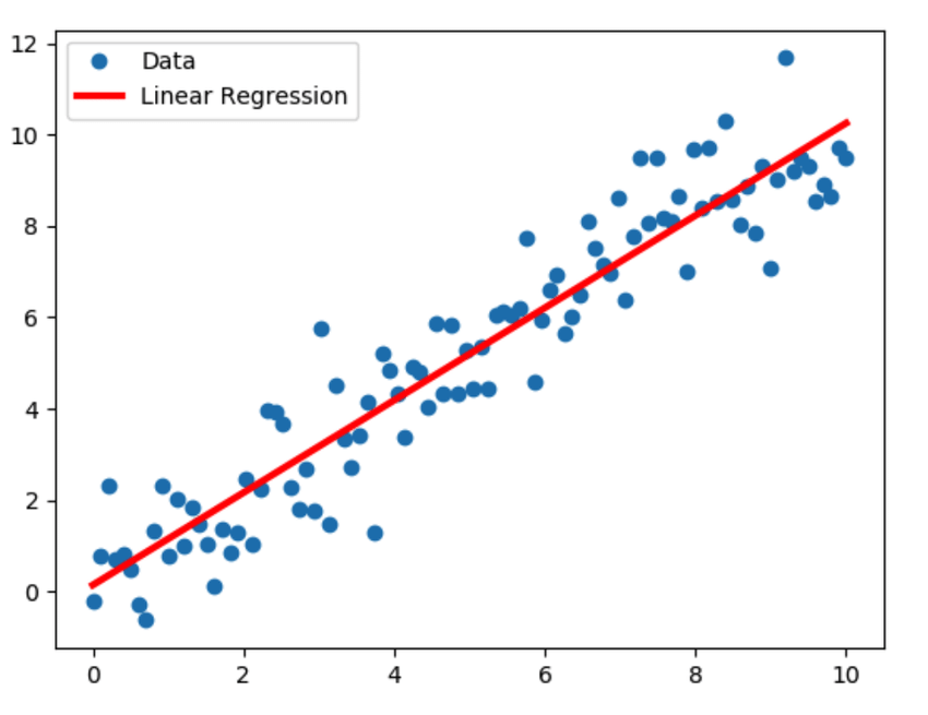
In this part, we will discuss more about the Supervised Model - Linear Regression. This model consists of fitting a straight line to our data that will predict the value. The straight line is calculated based on the training data provided.

When referring to the data, this notation is used: $(x^{(i)},y^{(i)})$ where i is the ith iteration of the test data used, x is the input, and y is the output.

With the training dataset and a learning algorithm, we will create a function that, when a new input value x is given, it calculates a result $\hat{y}$. This $\hat{y}$ wants to be as close to y (target value) as possible.

For the Linear Regression Model, the function is:

\[f_{w,b}(x) = wx + b\]

In Linear Regression, w is the slope of the line that the model will create.

Cost function formula

The cost function formula can tell us how the model is performing so we can upgrade it.

In machine learning, parameters of the model are the variables you can adjust during training to improve the model. In the Linear Regression model, the parameters are w and b. Parameters are also referred to as coefficients or weights.

Once we have our model $ f_{w,b}(x) $, we can use it to calculate $ \hat{y} $. A $ \hat{y}^{(i)} $ is obtained when using the model with the ith input:

\[\hat{y}^{(i)} = f_{w,b}(x^{(i)}) = wx^{(i)} + b\]

But we want $ \hat{y}^{(i)} $ to be close to $ y^{(i)} $ for all $ (x^{(i)},y^{(i)}) $, in other words, we want our model to predict a value that is close to the real value for each test data.

To measure how well our model is performing, we have to calculate the cost function (squared error cost function). To do this, we will calculate the square of all the errors obtained with the training examples:

\[J(w,b)=\frac 1 {2m} \sum_{i=1}^m (\hat{y}^{(i)} - y^{(i)})^2\]

This is the same as saying:

\[J(w,b)=\frac 1 {2m} \sum_{i=1}^m (f_{w,b}(x^{(i)}) - y^{(i)})^2\]

The goal is to minimize the value of this cost function $ J(w,b) $. If it is impossible to fit a single line that fits all the values, this cost will never reach 0. The 0 cost will only appear if it is possible to have a line that fits all the training data points.

If we wanted to plot this cost function for this case, since it has two parameters (w and b), the plot will have 3 dimensions. In this example image, assume that $ \theta_0 = 2$ and $ \theta_1 = b $.

Since we want to minimize the cost ($J(w,b)$), we would be aiming for a value that is at the bottom of this bowl.

We could also plot this in 2D as a function of w and b. In this plot, each line represents the same cost. You have to imagine it like the plot of the bowl has been cut horizontally and seen from above.

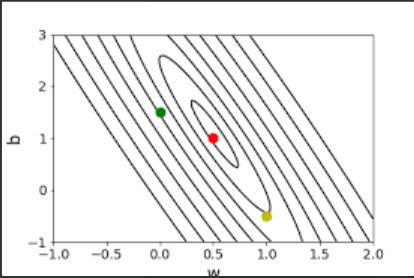
The red point in this plot implies a minimum (or low) cost, because the small circle represents the bottom of the bowl.

But, why when we are calculating the cost, we square the error? One reason is that the squared error function is differentiable and convex, meaning that it has a unique global minimum (minimum cost) that can be found using optimization techniques such as gradient descent. Additionally, squaring the error term helps to penalize larger errors more heavily, which is often desired in many applications.

Gradient descent

Ok, but how can we calculate the values of w and b that minimize the cost? The gradient descent algorithm can help us.

It works by iteratively adjusting the parameters of a model in the direction of the negative gradient of the cost function with respect to those parameters. In other words, it moves the model in the direction that most reduces the cost.

Following the linear regression example, we will have to adjust two parameters, w and b. They will be updated using this criteria:

Until they converge (the update is no longer noticeable):

\[w = w - \alpha \frac{\partial}{\partial w} J(w,b)\] \[b = b - \alpha \frac{\partial}{\partial b} J(w,b)\]

The $ \alpha $ is the learning rate, but we will talk about it later.

Bear in mind that if you are coding this, you don’t want b to get calculated using the new w. You will need to do something like this to avoid the problem:

\[temp\_w = w - \alpha \space \frac \partial {\partial w} J(w,b)\] \[temp\_b = b - \alpha \space \frac \partial {\partial b} J(w,b)\]

$ w = temp_w $

$ b = temp_b $

If we extend this function to calculate the derivatives, we will have this:

\[w = w - \alpha \frac{1}{2m} \sum_{i=1}^m (wx^{(i)} + b - y^{(i)}) 2x^{(i)} = w - \alpha \frac{1}{m} \sum_{i=1}^m (f_{w,b}(x^{(i)}) - y^{(i)}) x^{(i)}\] \[b = b - \alpha \frac{1}{2m} \sum_{i=1}^m (wx^{(i)} + b - y^{(i)}) 2 = w - \alpha \frac{1}{m} \sum_{i=1}^m (f_{w,b}(x^{(i)}) - y^{(i)})\]

Before talking about $\alpha$, I would like to explain why gradient descent works like this.

The parameters w and b are being updated by their actual value but subtracting the derivative value of the cost multiplied by the learning rate.

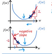
To understand the impact of this better, assume that we will only consider one parameter of the cost formula, so the plot will be in 2D. When we calculate the partial derivative of a function respect a relative point w, we are calculating the slope of that point. If the w is on the right side of the bowl plot, the slope will be positive, so the result of $\frac{\partial}{\partial w}J(w,b)$ will be positive. If we subtract a positive number from the actual w or b, the new values will be smaller (each iteration will be closer to 0, which is our goal).

However, if w is on the left side, the tangent line (slope) will have a negative value (second case in the image), the result $\frac{\partial}{\partial w}J(w,b)$ will be negative. Subtracting a negative number will increase the new values of w, which will produce a new cost closer to 0 too.

Keeping it short, updating w and b by subtracting their derivatives will give us new values that will imply a cost near 0.

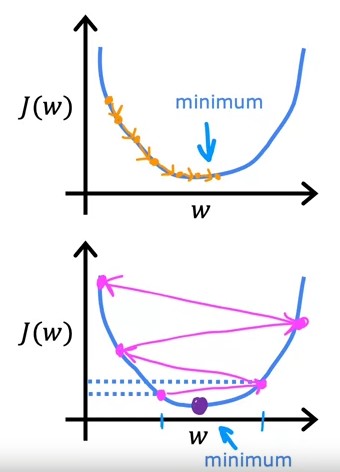
Now, let’s talk about $\alpha$ (learning rate). This value multiplies the value that we will use to update w and b. If we set a really low $\alpha$, each iteration of the gradient descent will update the values very slowly and it will take more iterations to reach the desired value. However, setting a large $\alpha$ is worse. If we heavily update the values, we may exceed the desired value and the cost will go from negative to positive values, increasing the absolute value (second case):

Now we know how to create a linear regression model and use the gradient descent function to obtain the best values to use in our model.

Logistic Regression

We are going to use Logistic Regression when the outcome is yes/no. We won’t predict a value with the given data, but decide if the given data is A or B (yes or no, positive or negative, etc.). One of the most used examples is to have the size of a tumor as input and decide if it is malignant or not.

Sigmoid function

To be able to do Logistic Regression, we first have to talk about the sigmoid function (logistic function). The shape of the function looks like this:

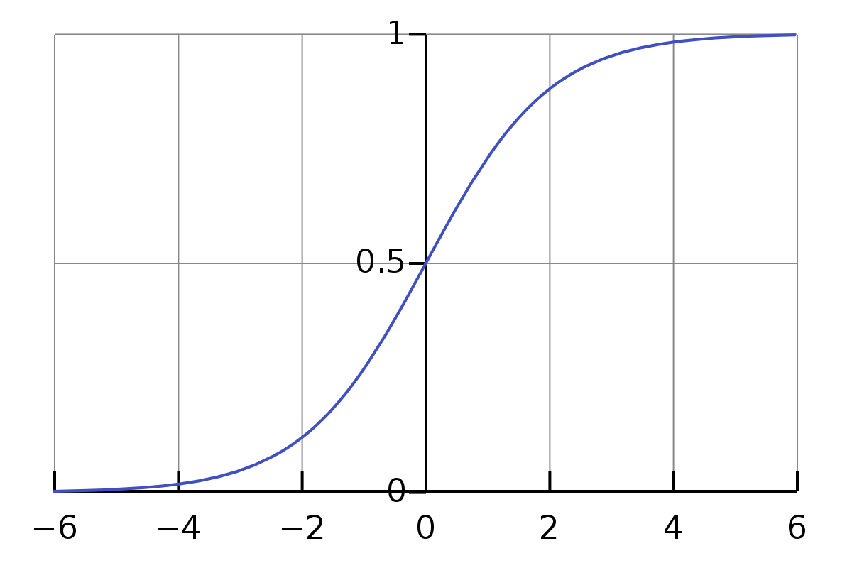
As you can see, all the values are between 0 and 1 (in the y-axis), where 0 is negative and 1 is positive. This is the sigmoid function:

$g(z) = \frac{1}{1+e^{-z}}$

But, what is $z$? $z$ is the value obtained when doing the linear regression explained in the other chapters:

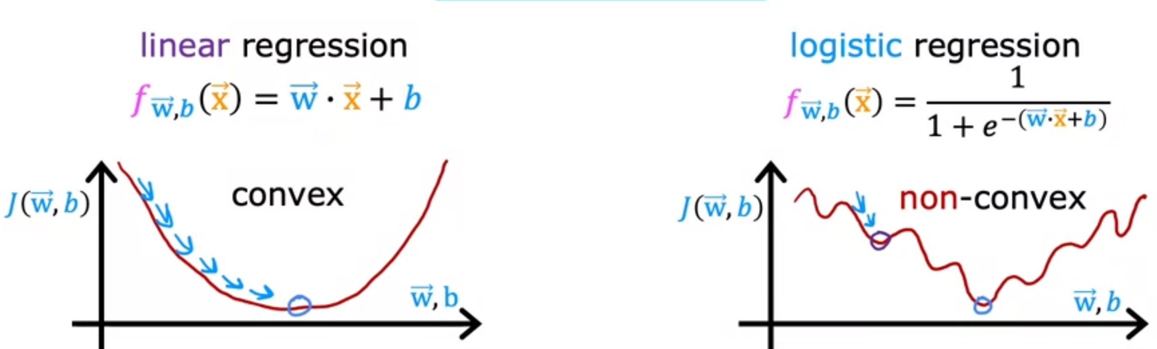
\[f_{\overrightarrow{w},b}(\overrightarrow{x}) = \overrightarrow{w} \cdot \overrightarrow{x} + b\]

This implies that:

$g(z) = g(\overrightarrow{w} \cdot \overrightarrow{x} + b) = \frac{1}{1+e^{-(\overrightarrow{w} \cdot \overrightarrow{x} + b)}}$

To sum up, this function will use the output obtained with the linear regression (multiple linear regression) function, with parameters $\overrightarrow{w}$ and $b$, and transform it into a value between 0 and 1.

Decision boundary

We said that 0 would be “negative” (which doesn’t mean bad) and 1 positive. However, when using the sigmoid function, we will probably obtain values between these two numbers. We need to define a decision boundary that defines when it is considered 0 and when it is considered 1. Another way to interpret this is the probability that $y=1$ given $x$ and parameterized by $w$ and $b$:

\[f_{\overrightarrow{w},b}(\overrightarrow{x}) = P(y=1|x;\overrightarrow{w},b)\]

Assuming that we will predict that $\hat{y} = 1$ when $f_{\overrightarrow{w},b}(\overrightarrow{x})$ (logistic regression function) $\geq 0.5$, this implies the following:

$f_{\overrightarrow{w},b}(\overrightarrow{x})$ will be $\geq 0.5$ if $g(z) \geq 0.5$ because $f_{\overrightarrow{w},b}(\overrightarrow{x}) = g(z)$.

Since $g(z) = \frac{1}{1+e^{-(\overrightarrow{w} \cdot \overrightarrow{x} + b)}}$, it will be $\geq 0.5$ whenever $z \geq 0$.

Since $z = \overrightarrow{w} \cdot \overrightarrow{x} + b$, it will be $\geq 0$ whenever $\overrightarrow{w} \cdot \overrightarrow{x} + b$ is $\geq 0$.

Having stated this, we could plot the decision boundary doing this (in this example where the threshold is 0.5):

$z = \overrightarrow{w} · \overrightarrow{x} + b = 0$

Cost function

We can’t use the same cost function method with logistic regression because when doing the gradient descent, we wouldn’t have a convex function and we would not be able to find the minimum local value (there would be several local values).

Remember, that for liniar regression, the cost function was

$J(w,b)=\frac 1 {2m} \sum_{i=1}^m (f_{w,b}(x^{(i)}) - y^{(i)})^2$

But since this function won’t work when doing logistic regression, we have to find anothre way. The cost function for the logistic regression looks like this:

$J(\mathbf{w},b) = \frac{1}{m} \sum_{i=0}^{m-1} \left[ L(f_{\mathbf{w},b}(\mathbf{x}^{(i)}), y^{(i)}) \right]$

We will first define the new term Loss. Loss is a measure of the difference of a single example to its target value (the cost for a single data point):

$L(f_{w,b}(x^{(i)}), y^{(i)})$

Going back again to the logistic regression, the Loss would be

$L(f_{w,b}(x^{(i)}), y^{(i)}) = (f_{w,b}(x^{(i)}) - y^{(i)})^2$

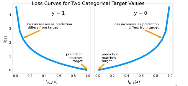
However, for the logistic regression, we will have this (The loss function will be different depending on the target value $y^{(i)}$):

\[L(f_{w,b}(x^{(i)}), y^{(i)}) = \begin{cases} -log(f_{w,b}(x^{(i)}) &\text{if } y^{(i)}= 1 \\ -log(1 - f_{w,b}(x^{(i)}) &\text{if } y^{(i)}= 0 \end{cases}\]

Plotting this we can see that we obtain a way to calculate a cost that can be enhanced using gradient descent.

Another way to rewrite this Loss function in a simplified single expression is this one:

$L(f_{\mathbf{w},b}\mathbf{x}^{(i)}), y^{(i)}) = -y^{(i)} \log(f_{\mathbf{w},b}( \mathbf{x}^{(i)} ) ) - ( 1 - y^{(i)}) \log ( 1 - f_{\mathbf{w},b}( \mathbf{x}^{(i)} ) )$

Since $y^{(i)}$ can be 1 or 0,

If $y^{(i)} = 0$ the first part is eliminated:

$(-(0) \log\left(f_{\mathbf{w},b}\left( \mathbf{x}^{(i)} \right) \right) - \left( 1 - 0\right) \log \left( 1 - f_{\mathbf{w},b}\left( \mathbf{x}^{(i)} \right) \right) = -\log \left( 1 - f_{\mathbf{w},b}\left( \mathbf{x}^{(i)} \right) \right)$

If $y^{(i)} = 1$ the second part is eliminated:

$(-(1) \log\left(f_{\mathbf{w},b}\left( \mathbf{x}^{(i)} \right) \right) - \left( 1 - 1\right) \log \left( 1 - f_{\mathbf{w},b}\left( \mathbf{x}^{(i)} \right) \right) = -\log\left(f_{\mathbf{w},b}\left( \mathbf{x}^{(i)} \right) \right)$

Since all is going to be negative values, we can extract the negative and put it in front of the Cost function instead of the Loss function.

$J(\mathbf{w},b) =- \frac{1}{m} \sum_{i=0}^{m-1} [y^{(i)} \log(f_{\mathbf{w},b}( \mathbf{x}^{(i)} ) ) + ( 1 - y^{(i)}) \log ( 1 - f_{\mathbf{w},b}( \mathbf{x}^{(i)} ) )]$

Gradient Descent in Logistic Regression

The gradient descent algorithm works the same as in the Linear Regression.

Until they converge:

$w_j = w_j - \alpha \space \frac \partial {\partial w_j} J(w,b)$

$b = b - \alpha \space \frac \partial {\partial b} J(\overrightarrow{w},b)$

And the derivatives remain the same as the Linear Regression:

$\frac \partial {\partial w_j} J(w,b) = \frac 1 {m} \sum_{i=1}^m (f_{w,b}(x^{(i)}) - y^{(i)}) \space x^{(i)}$

$\frac \partial {\partial b} J(\overrightarrow{w},b) = \frac 1 {m} \sum_{i=1}^m (f_{w,b}(x^{(i)}) - y^{(i)})$

Even though it looks like the formula is the same, the function $f_{w,b}(x^{(i)})$ is different in this Logisitic Regression

Multiple Linear Regression

When we were explaining the Linear Regression in the last post, we were only using one variable (the had only one feature). In this post we will see the situation where the input variable has several features.

If the input variable has more than one feature, we can say that is a vector and represent it like this:

$\overrightarrow{x} = [x_1, x_2, x_3, … , x_n]$

If we say $x_2$ we are saying referring to the second feature. If we are saying $x_3^4$ we are making reference to the third feature of the fourth training example.

Now, the liniar regression model can be represented differently. Here you can ser both models to identify the differences.

Linear Regression

$f_{w,b}(x) = wx + b$

Multiple Linear Regression

$f_{\overrightarrow{w},b}(\overrightarrow{x}) = \overrightarrow{w}·\overrightarrow{x} + b = w_1x_1 + w_2x_2 + … + w_n+x_n + b = (\sum_{j=1}^n w_jx_j) + b$

You can see that w is now represented as $\overrightarrow{w}$ too. This implies that it will be a vector too. Each feature $x_i$ will have its own parameter $w_i$.

Gradient descent for multiple linear regression

The new cost function uses the vector notation for the w parameters:

$J(\overrightarrow{w},b)$

In the gradient descent algorithm for one feature, we just had to calculate the new values for w and b and then update them simultaneously. However, now w is a vector and we need to update all the parameters with it’s corresponding $x_i$

Gradient descent in a normal linear regression:

$w = w - \alpha \space \frac 1 {m} \sum_{i=1}^m (f_{w,b}(x^{(i)}) - y^{(i)}) \space x^{(i)}$

Gradient descent in multiple linear regression:

$w_j = w_j - \alpha \space \frac 1 {m} \sum_{i=1}^m (f_{\overrightarrow{w},b}(\overrightarrow{x}^{(i)}) - y^{(i)}) \space x_j^{(i)} \space for \space j = 0…n-1$

$b = b - \alpha \space \frac 1 {m} \sum_{i=1}^m (f_{\overrightarrow{w},b}(\overrightarrow{x}^{(i)}) - y^{(i)})$

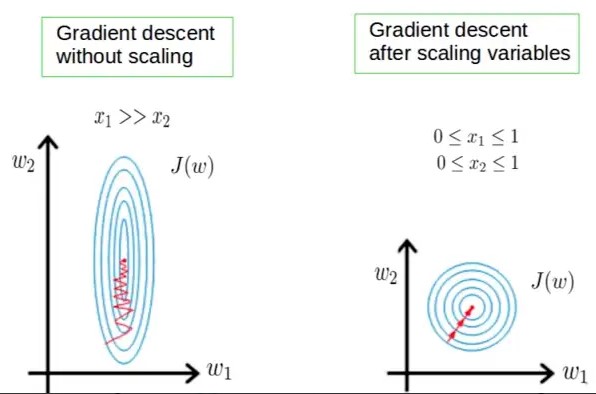
Feature scaling

In a multiple linear regression model, feature scaling is a technique used to standardize the range of independent variables or features of the data. We aim to normalize the features between the range of -1 and 1.

For example, consider a dataset with two features, “house area” and “number of rooms”. The “house area” feature has a range of values from 1000 to 2500 square feet, while the “number of rooms” feature has a range of values from 2 to 5 rooms. Without feature scaling, the optimization algorithm used to find the optimal coefficients of the model would be affected by the difference in scales between these two features, leading to slow convergence or the model gets stuck in local optima.

Another example, consider a dataset with two features, “income” and “age”, the “income” feature has a range of values from $20,000 to $200,000 while the “age” feature has a range of values from 18 to 70. Without feature scaling, the “income” feature could dominate the model, meaning that it would have a larger influence on the model’s predictions than the “age” feature. This could lead to a model that is not well-balanced and may not generalize well to new data.

By applying feature scaling, these examples can be transformed into the same scale, allowing the optimization algorithm to converge faster and preventing features with larger scales from dominating the model. Common techniques for feature scaling include min-max scaling and standardization.

We can scale features in different ways, like mean normalization (also known as min-max normalization) or z-score normalization (also known as Standardization).

Mean normalization

In mean normalization, we want to normalize the features between -1 and 1 (approximately). The formula to obtain the normalized feature is:

$x_j^{(i)} = \frac {x_j^{(i)} - \mu_j} {max_j - min_j}$

Where:

$x_j^{(i)}$ is the feature $j$ of the training example $i$ that we want to normalize

$\mu_j$ is the mean of the feature $j$ calculated using all (m) training examples $\mu_j = \frac {\sum_{i=1}^m x_j^{(i)}} m$

$max_j$ is the max value of $x_j$ between all training examples.

$min_j$ is the min value of $x_j$ between all training examples.

Z-score normalization

In order to compute this normalization, we need to obtain the standard deviation for the feature j:

$\sigma_j = \sqrt{\frac{1}{m} \sum_{i=0}^{m-1} (x^{(i)}_j - \mu_j)^2}$

Then we can use this formula:

$x^{(i)}_j = \dfrac{x^{(i)}_j - \mu_j}{\sigma_j}$

There is no need to normalize all the features. If a feature already ranges between -3 and 3, there is no need to rescale. We should rescale always that the features are really large or really small.

Polinomial regression

Linear regression consists of the creation of a straight line, however, this line won’t always fit correctly the model since there are situations where the results don’t tend to be linear.

In this situation, we can use feature engineering and modify our features with polynomials in order to make the model predict no linear situations.

In this first example, the predicted value is obtained using the normal linear regression model:

$f_{w,b}(x) = wx + b$

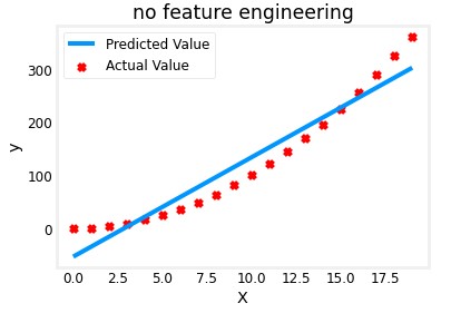
As you can see, it doesn’t fit the actual values really well. If we make use of feature engineering and modify the features creating a new one where $x$ is modified to $x^2$, the model would look like this:

$f_{w,b}(x) = wx^2 + b$

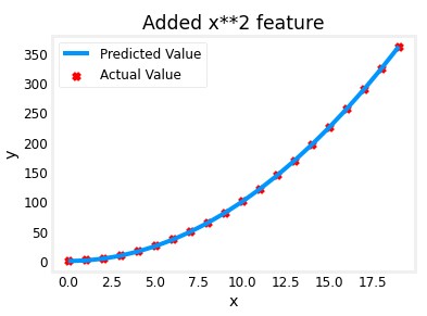
Thanks to the gradient descent that will adjust the correct value for each $w_j$ (it will set really low values for features that are not important), we can model complex functions to fit the non linear values.

Programming a Multiple Linear Regression

Let’s make a practical example. We will build a model that predicts the house price taking into consideration the size, number of bedrooms, number of floors and the age of the house.

Training data

We will use this training examples:

Size	Number of Bedrooms	Number of Floors	Age of Home	Price
2104	5	1	45	460
1416	3	2	40	232
852	2	1	35	178

We will add all the “features” in a numpy array and the prices in another one (the features are $x$ and the price is $y$)

X_train = np.array([[2104, 5, 1, 45], [1416, 3, 2, 40], [852, 2, 1, 35]])
y_train = np.array([460, 232, 178])

You can notice that in X_train, the X is in uppercase. Since being a 2-D array, we consider it a matrix and in algebra matrix are represented in uppercase.

$\mathbf{X} = \begin{Bmatrix} x_0^{(0)} & x_1^{(0)} & … & x_{n-1}^{(0)}
x_0^{(1)} & x_1^{(1)} & … & x_{n-1}^{(1)}
…
x_0^{(m-1)} & x_1^{(m-1)} & … & x_{n-1}^{(m-1)} \end{Bmatrix}$

$x^{(i)}$ is the vector containing the example i. For example, $x^{(0)}$ is the first vector example, assuming that the examples are the ones of the table above, $x^{(0)} = (2104, 5, 1, 45)$

$x_j^{(i)}$ is element j in example i. Using the same example, $x_0^{(0)} = 2104$

Parameters w and b

As mentioned previously, since we have different features, we will have a $w_n$ for each one. Since in this example n = 4 (we have 4 features), $w$ will be a 1-D array with 4 parameters.

$b$ remains as scalar.

We can guess some initial values for this parameter since they will be adjusted when doing the gradient descent:

b_init = 785.1811367994083
w_init = np.array([ 0.39133535, 18.75376741, -53.36032453, -26.42131618])

Cost

Now we will compute the cost obtained with the values that we invented for the parameters w and b. The formula of the cost was:

$J(\mathbf{w},b) = \frac{1}{2m} \sum\limits_{i = 0}^{m-1} (f_{\mathbf{w},b}(\mathbf{x}^{(i)}) - y^{(i)})^2$ where:

$f_{\mathbf{w},b}(\mathbf{x}^{(i)}) = \mathbf{w} \cdot \mathbf{x}^{(i)} + b$

In python, we could compute the cost using a code like this:

def compute_cost(X, y, w, b): 
    m = X.shape[0]
    cost = 0.0
    for i in range(m):                                
        f_wb_i = np.dot(X[i], w) + b           #(n,)(n,) = scalar
        cost = cost + (f_wb_i - y[i])**2       #scalar
    cost = cost / (2 * m)                      #scalar    
    return cost

cost = compute_cost(X_train, y_train, w_init, b_init)
#cost = 1.5578904045996674e-12

Gradient Descent

Remember that for calculating the gradient descent we have to follow this formula:

$w_j = w_j - \alpha \space \frac{\partial J(\mathbf{w},b)}{\partial w_j}$

$b = b - \alpha \space \frac{\partial J(\mathbf{w},b)}{\partial b}$

We can create a function to compute the derivative part of the gradient descent:

$\frac{\partial J(\mathbf{w},b)}{\partial w_j} = \frac{1}{m} \sum\limits_{i = 0}^{m-1} (f_{\mathbf{w},b}(\mathbf{x}^{(i)}) - y^{(i)})x_{j}^{(i)}$ $\frac{\partial J(\mathbf{w},b)}{\partial b} = \frac{1}{m} \sum\limits_{i = 0}^{m-1} (f_{\mathbf{w},b}(\mathbf{x}^{(i)}) - y^{(i)})$

def compute_gradient(X, y, w, b): 

    m,n = X.shape           #(number of examples, number of features)
    dj_dw = np.zeros((n,))
    dj_db = 0.

    for i in range(m):                             
        err = (np.dot(X[i], w) + b) - y[i]   
        for j in range(n):                         
            dj_dw[j] = dj_dw[j] + err * X[i, j]    
        dj_db = dj_db + err                        
    dj_dw = dj_dw / m                                
    dj_db = dj_db / m                                
        
    return dj_db, dj_dw
tmp_dj_db, tmp_dj_dw = compute_gradient(X_train, y_train, w_init, b_init)

Now we can compute the gradient descent using this code:

def gradient_descent(X, y, w_in, b_in, cost_function, gradient_function, alpha, num_iters): 
    w = copy.deepcopy(w_in)  #avoid modifying global w within function
    b = b_in
    
    for i in range(num_iters)
        # Calculate the gradient and update the parameters
        dj_db,dj_dw = gradient_function(X, y, w, b)   ##None

        # Update Parameters using w, b, alpha and gradient
        w = w - alpha * dj_dw               ##None
        b = b - alpha * dj_db               ##None

    return w, b

Numpy Basics

NumPy is a library that extends the base capabilities of python to add a richer data set, including more numeric types, vectors, matrices, and many matrix functions.

Numpy Arrays

In algebra, the number of elements of the vector can be referred as dimension or rank, however, in numpy arrays, the dimension is the number of indexes of an array.

#This numpy array is a 1-D (one dimension), shape (3,) array, with the elements indexed [0] through [2]: 
n = np.array([10, 20, 30])

#This numpy array is a 2-D (two dimensions, or Matrices), shape (2, 3) array, with the elements indexed [0][0] through [1][2]: 
n2 = np.array([[1,3,5],[4,8,12]])

#This numpy array is a 3-D (three dimensions), shape (2, 2, 3) array, with the elements indexed [0][0][0] through [1][1][2]: 
n3 = np.array([[[1,2,3],[4,5,6]],[[7,8,9],[10,11,12]]])

Data creation routines in NumPy will generally have a first parameter which is the shape of the object. This can either be a single value for a 1-D result or a tuple (n,m,…) specifying the shape of the result. However, values can be specified manually as shown in the example above.

Indexing and Slicing

Elements of vectors can be accessed via indexing and slicing.

Indexing: means referring to an element of an array by its position within the array.

#vector indexing operations on 1-D vectors
a = np.arange(10)
print(a)
#Output: [0 1 2 3 4 5 6 7 8 9]

print(a[2])
#Output: 2

# access the last element, negative indexes count from the end
print(a[-1])
#Output: 9

Slicing: means getting a subset of elements from an array based on their indices. It creates an array of indices using a set of three values (start:stop:step). A subset of values is also valid.

#vector slicing operations
a = np.arange(10)
print(a)
#Output: [0 1 2 3 4 5 6 7 8 9]

#access 5 consecutive elements (start:stop:step)
c = a[2:7:1];
print(c)
#Output: [2 3 4 5 6]

# access 3 elements separated by two 
c = a[2:7:2];
print(c)
#Output: [2 4 6]

# access all elements index 3 and above
c = a[3:];
print(c)
#Output: [3 4 5 6 7 8 9]

# access all elements below index 3
c = a[:3];
print(c)
#Output: [0 1 2]

# access all elements
c = a[:];
print(c)
#Output: [0 1 2 3 4 5 6 7 8 9]

Single Vector Operations

You can do several operations with one single vector like:

a = np.array([1,2,3,4])
print(a)
#Output: [1,2,3,4]

#Negate all elements
b = -a

#Sum all elements
b = np.sum(a)

#Do the mean of all elements 
b = np.mean(a)

#square up all elements
b = a**2

Vector Vector Operations

Most arithmetic, logical and comparison operations that NumPy have can be applied to vectors, but they must be the same size.

a = np.array([ 1, 2, 3, 4])
b = np.array([-1,-2, 3, 4])
print(a + b)
#Output: [0 0 6 8]

Scalar Vector Operations

You can also apply arithmetic operations with a single scalar value and a vector.

a = np.array([1, 2, 3, 4])

# multiply a by a scalar
b = 5 * a
print(b)
#Output: [ 5 10 15 20]

Vector Dot Product

The dot product of two vectors is not the same as multiply two vectors. Is the sum the results obtained by multiplying each value for the value with the same index of the other vector.

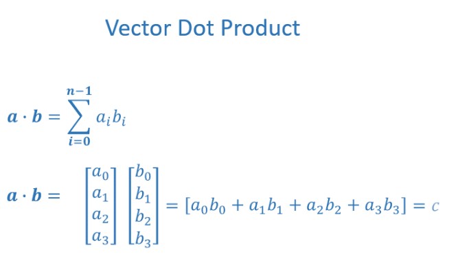
Here you can see the difference:

a = np.array([ 1, 2, 3, 4])
b = np.array([-1,-2, 3, 4])

#Normal Multiplication
print(a*b)
#Output: [-1 -4  9 16]

#Dot Product
print(np.dot(a,b))
#Output: 20

We could implement the dot product by coding this for loop:

def example_dot(a, b): 
    x=0
    for i in range(a.shape[0]):
        x = x + a[i] * b[i]
    return x

a = np.array([1, 2, 3, 4])
b = np.array([-1, -2, 3, 4])
print(example_dot(a, b))

#Output: 20

However, using the np.dot(a,b) is more efficient because it uses parallelization.

Overfitting and Regularization

Overfitting is a common problem in machine learning where a model is trained too well on the training data, to the point where it starts to fit to the noise or random fluctuations in the data, rather than capturing the underlying patterns and relationships.

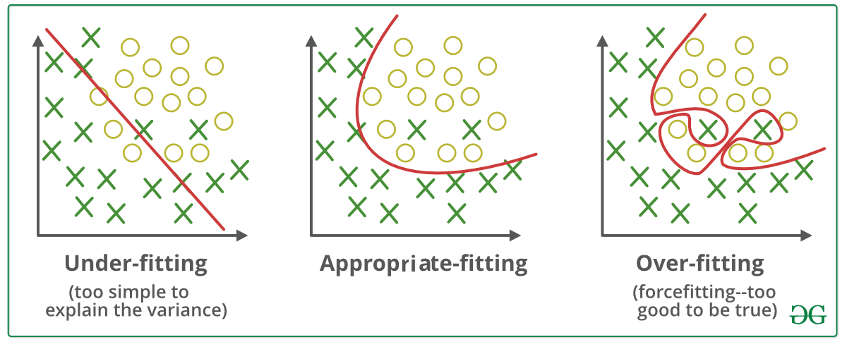
A way to solve this overfitting when models are high polynomial functions is to use Regularitzation. What regularization does is to encourage smaller weights ($w_j$) by adding a “penalty term” to the loss function while training the model.

Loss function for Liniar Regression with Regularitzation

The Loss function with regularization is the next one:

$J(w,b)=\frac 1 {2m} \sum_{i=1}^m (f_{w,b}(x^{(i)}) - y^{(i)})^2$ $+ \frac \lambda {2m} \sum_{j=1}^n w_j^2$

If $\lambda$ (the learning rate) is too big, the function will underfit, if it is too small, the penalization won’t be enough and the model will overffit.

Now, when doing the gradient descent, the expressions also have to consider this penalty term:

$\frac \partial {\partial w_j} J(w,b) = \frac 1 {m} \sum_{i=1}^m (f_{w,b}(x^{(i)}) - y^{(i)}) \space x^{(i)}$ $+ \frac \lambda {m} w_j$

$\frac \partial {\partial b} J(\overrightarrow{w},b) = \frac 1 {m} \sum_{i=1}^m (f_{w,b}(x^{(i)}) - y^{(i)})$

So, the gradient descent algorithm is:

repeat until they converge:

$w_j = w_j - \alpha [\frac 1 {m} \sum_{i=1}^m [(f_{w,b}(x^{(i)}) - y^{(i)}) \space x^{(i)}] + \frac \lambda {m} w_j]$

$b = b - \alpha \frac 1 {m} \sum_{i=1}^m (f_{w,b}(x^{(i)}) - y^{(i)})$

Loss function for Logistic Regression with Regularitzation

It just works the same for Logistic Regression. We are going to add the same penalty value to the loss function.

$J(\mathbf{w},b) =- \frac{1}{m} \sum_{i=0}^{m-1} [y^{(i)} \log(f_{\mathbf{w},b}( \mathbf{x}^{(i)} ) ) - ( 1 - y^{(i)}) \log ( 1 - f_{\mathbf{w},b}( \mathbf{x}^{(i)} ) )]$ $+ \frac \lambda {m} w_j$

As mentioned in the previous chapter, the Gradient descent function with Logistic Regression looks the same but the $f_{\mathbf{w},b}( \mathbf{x}^{(i)} )$ is different. However, they can be represented identically:

Until they converge:

$w_j = w_j - \alpha [\frac 1 {m} \sum_{i=1}^m [(f_{w,b}(x^{(i)}) - y^{(i)}) \space x^{(i)}] + \frac \lambda {m} w_j]$

$b = b - \alpha \frac 1 {m} \sum_{i=1}^m (f_{w,b}(x^{(i)}) - y^{(i)})$