NLP-1: Logistic Regression

Natural Language Processing or NLP is a branch of artificial intelligence that enables machines to understand, interpret, and generate human language. With the growing volume of textual data available, NLP has become a critical tool for businesses, researchers, and individuals.

In this blog series, we will explore the basics of NLP, from the underlying concepts and techniques to the tools and applications used in the field.

Logistic Regression in NLP

In this section, we will learn how to use the Logistic Regression Model to classify text as having a positive or negative sentiment.

Since we have already explained how logistic regression works in a previous post, we will avoid repeating the same concepts here.

Vocabulary

First we will learn how to represent text as a vector. The first step is to create a Vocabulary. A vocabulary refers to the set of unique words or terms that are used in a particular text input/corpus, document, or language. A vocabulary is essentially a collection of all the words or terms that occur in a given set of text data, along with their respective frequencies of occurrence.

Suppose we have a collection of three short sentences:

1. The cat sat on the mat.
2. The dog chased the cat.
3. The cat ran away from the dog.

The vocabulary for this text input would consist of all the unique words that appear in the sentences, along with their respective frequencies of occurrence. Here’s what the vocabulary might look like: {“The”: 3, “cat”: 3, “sat”: 1, “on”: 1, “the”: 3, “mat”: 1, “dog”: 2, “chased”: 1, “ran”: 1, “away”: 1, “from”: 1}

Once we have a vocabulary, we can represent a text as a vector by setting 1 for the words in the vocabulary that appear in the text and 0 for the words that aren’t in the text. Continuing with the same example, using the vocabulary:

{“The”, “cat”, “sat”, “on”, “the”, “mat”, “dog”, “chased”, “ran”, “away”, “from”}

and the text:

“The cat sat on the mat”.

We can find the vector 1111110000:

The	cat	sat	on	the	mat	dog	chased	ran	away	from
1	1	1	1	1	1	0	0	0	0	0

As you can imagine, the longer the vocabulary, the longer the vectors will be (with a lot of 0 values). This will result in a longer training time and prediction time.

Frequency Dictionary

The next step is to create a frequency dictionary using the vocabulary. Let’s do a new example related to our objective of being able to classify text as having a positive or negative sentiment. We have this text corpus and we classify each sentence as positive or negative:

1. I am happy to see you (positive (1)
2. I am sad (negative (0)
3. Today I feel happy (positive (1)
4. This was a sad moment of my life (negative (0)

Then we can create this vocabulary:

{”I”,”am”, “happy”, “to”, “see”, “you”, “sad”, “Today”, “feel”, “This”, “was”, “a”, “moment”, “of”, “my”, “life”}

Now, since we have the sentences classified as positive or negative, we can create a frequency dictionary for positive text and negative text. A frequency dictionary is the vocabulary but with the frequency of each word in a sentence categorized as positive or negative (in this example).

The positive (1) frequency dictionary with the previous example would be:

 {”I”: 2,”am”: 1, “happy”: 2, “to”: 1, “see”: 1, “you” : 1, “sad”: 0, “Today”: 1, “feel”: 1, “This”: 0, “was”: 0, “a”: 0, “moment”: 0, “of”: 0, “my”: 0, “life”: 0}

The negative (0) frequency dictionary with the previous example would be:

 {”I”: 1,”am”: 1, “happy”: 0, “to”: 0, “see”: 0, “you” : 0, “sad”: 2, “Today”: 0, “feel”: 0, “This”: 1, “was”: 1, “a”: 1, “moment”: 1, “of”: 1, “my”: 1, “life”: 1}

We can use these frequency dictionaries that we just created to represent any tweet as a 3-dimensional vector. To do this, we will use this expression:

$X_m = [1,\sum_wfreqs(w,1), \sum_wfreqs(w,0)]$

This expresion means that the features of a text m has the value 1 for the first dimension (bias), the sum of positive frequencies from the positive frequency dictionary for each word of the text for the second dimension, and the sum of negative frequencies from the negative frequency dictionary for each word of the text for the third dimension.

Bearing in mind the two frequency dictionaries exposed above as example, the text:

Today I feel happy

Would be represented as:

$X_1 = [1,6,1]$

This improves the previous representation of a text where the vector had the same dimension as the vocabulary.

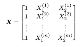
If we obtain this vector for several twitts (m), we will end up with a $m$x$3$ matrix.

Text Preprocessing

Let’s take a step back and imagine a new example. In this case, imagine that the text corpus consists of tweets. We could have texts like this one:

OMG!! Yesterday I was feeling BAD. I think I may be sick!!

We should apply some preprocessing before analyzing or creating a vocabulary using this corpus. There are different ways of preprocessing.

Stop words and punctuation

Using some dictionaries we can remove words like {”and”,”is”,”are”,”at”,be”, “has”,”for”, …} that doesn’t add a lot of meaning to the sentence. This words are known as stop words.

In addition, we can remove punctuation marks using another dictionary like {”,”, “.”, “:”, “!”, “?”, …}

Using this two preprocessing steps, the example twitt can be processed to this one:

OMG Yesterday feeling BAD think sick

You can see that we are able to keep understanding the meaning of what the twitt is about.

Steaming and Lowercasing

We can even process the tweet a bit more. Stemming is the process of reducing a word to its base or root form, known as the stem. This process involves removing suffixes and prefixes from a word to obtain the core meaning of the word. For example, the stem of the word “jumping” is “jump”, and the stem of the word “dogs” is “dog”.

Lowercasing is the process of reducing all text to lowercase, so we avoid having different values in a vocabulary corresponding to the same word, such as “OMG” and “omg”.

If we apply stemming and lowercasing to the previously processed example, we get this final result:

omg yesterday feel bad think sick

Here you can see the whole transformation and how the text input is reduced and simplified:

OMG!! Yesterday I was feeling BAD. I think I may be sick!! —> omg yesterday feel bad think sick

Applying Logistic Regression

Remember that the logistic regression formula was:

$g(z) = \frac{1}{1+e^{-z}}$

However, now z will be:

$\theta^T x^{(i)}$

where $\theta$ is a vector of parameters that must be trained. So the final expression is:

$h(x^{(i)},\theta) = \frac{1}{1+e^{-\theta^T x^{(i)}}}$

$x^{(i)}$ is the 3-dimensional vector obtained with the frequency dictionary.

Remember that $\theta$ should be trained using gradient descent. The cost function that should be used is the same as the one explained in the Logistic Regression chapter. However, the expression should now contain $\theta$:

$J(\theta) =- \frac{1}{m} \sum_{i=0}^{m-1} [y^{(i)} \log h(x^{(i)},\theta) + ( 1 - y^{(i)}) \log ( 1 - h(x^{(i)},\theta) )]$

Since we are using matrix, we could vectorize this expression as:

$J(θ)=\frac1 m⋅−y^Tlog⁡(h)−(1−y)^Tlog⁡(1−h)$

And the gradient descent update step expression:

Repeat{

$θ_j:=θ_j− \frac α m ∑_{i=1}^m(h(x^{(i)},θ)−y^{(i)})x_j^{(i)}$

}

Once the $\theta$ has been trained, we can guess the sentiment of a new corpus by representing it as a vector and applying the logistic regression. If it is > 0.5 it can be classified as positive.