
NLP with Naive Bayes’
Naive Bayes’ theorem is a statistical algorithm that is widely used in natural language processing (NLP) to perform classification tasks, such as sentiment analysis, text categorization, and spam detection. Naive Bayes is a probabilistic model that makes predictions based on the probabilities of different features occurring in a given text.
Naive Bayes’ theorem is based on Bayes’ theorem, which states that the probability of an event occurring given some prior knowledge is proportional to the probability of that knowledge given the event. In NLP, the event is typically the occurrence of certain words or phrases in a text, and the prior knowledge is the probability of these words occurring in texts belonging to different categories.
The “naive” part of Naive Bayes comes from the assumption that the features (words or phrases) in a text are conditionally independent of each other given the category. This assumption simplifies the calculation of probabilities and allows the algorithm to be applied to large datasets with many features.
Understanding Bayes’ Rule
In order to understand Bayes’ Rule, we need to understand what Conditional Probability is. Conditional probability is a measure of the probability of an event occurring, given that another event has already occurred. In other words, it is the probability of event A given that event B has occurred. It is denoted as \(P(A | B)\), where “|” means “given that” and “A” and “B” are events.
The formula for conditional probability is:
\[P(A | B) = \frac {P(A \cap B)} {P(B)}\]where \(P(A \cap B)\) is the probability of both events A and B occurring, and \(P(B)\) is the probability of event B occurring.
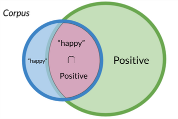
Using the example of the probability of a tweet being positive if it contains the word “happy”, we can express it as:
\[P(Positive | “happy”) = \frac {P(Positive \cap “happy”)} {P(”happy”)}\]And if we wanted to represent the probability of a tweet containing the word “happy” if it is positive, the expression would look like this:
\[P(“happy”| Positive) = \frac {P(“happy”\cap Positive)} {P(Positive)}\]Knowing that ${P(“happy”\cap Positive)} = {P(Positive\cap “happy”)}$ because they represent the same space:
We can reach the conclusion (by doing some algebra) that:
\[P(Positive | “happy”) = P(”happy” | Positive) \times \frac {P(Positive)} {P(”happy”)}\]The denominator $P(“happy”)$ (in this example) is usually treated as a constant factor that can be ignored when comparing the posterior probabilities of different labels (e.g., positive vs. negative) for the same input text. This is because the denominator P(“happy”) is the same for both labels and does not affect the relative probabilities of the labels given the input text. Therefore, it can be omitted from the calculation and the label with the highest posterior probability can be selected as the predicted label.
In practice, the denominator P(“happy”) is often estimated using some smoothing technique to avoid zero probabilities for words that do not appear in the training data. We will see one of this soothing rechniques later. So, in other words, the Bayes’ rule we can calculate the probability of $ P(A | B) $ if we already know the probability of \(P(B | A)\) and their ratios ( \(P(A)\) and \(P(B)\) ):
\[P(A | B) = \frac {P(B | A)P(A)} {P(B)}\]Applying Naive Bayes’ in NLP
Retrieving the example we used in Logistic Regression:
- I am happy to see you (positive (1)
- I am sad (negative (0)
- Today I feel happy (positive (1)
- This was a sad moment of my life (negative (0)
We can create the following frequency tables:
| Values | Positive Frequency | Negative Frequency |
|---|---|---|
| I | 2 | 1 |
| am | 1 | 1 |
| happy | 2 | 0 |
| to | 1 | 0 |
| see | 1 | 0 |
| you | 1 | 0 |
| sad | 0 | 2 |
| Today | 1 | 0 |
| feel | 1 | 0 |
| This | 0 | 1 |
| was | 0 | 1 |
| a | 0 | 1 |
| moment | 0 | 1 |
| of | 0 | 1 |
| my | 0 | 1 |
| life | 0 | 1 |
| Total: | 10 | 11 |
This allows us to create the same table but instead of frequency, with probabilities for each word being in a positive or negative tweet. To do this, we have to pick each word and divide its’ frequency in a positive/negative context for the total words of that context. For example, the probability of word I being in a Positive tweet P(”I”|Positive) is: $2/10 = 0.2$
Here I provide the whole table:
| Values | Positive Probability | Negative Probability |
|---|---|---|
| I | 0.2 | 0.1111 |
| am | 0.1 | 0.1111 |
| happy | 0.2 | 0 |
| to | 0.1 | 0 |
| see | 0.1 | 0 |
| you | 0.1 | 0 |
| sad | 0 | 0.2222 |
| Today | 0.1 | 0 |
| feel | 0.1 | 0 |
| This | 0 | 0.1111 |
| was | 0 | 0.1111 |
| a | 0 | 0.1111 |
| moment | 0 | 0.1111 |
| of | 0 | 0.1111 |
| my | 0 | 0.1111 |
| life | 0 | 0.1111 |
When we obtain this table, values that have the same probability in both columns don’t provide any value and could be ignored.
Now that we have this table, we could compute the likelihood of a new tweet following this expression, where $w_i$ represents the ith word of the corpus and $m$ the total amount of words that the corpus has:
\[\prod_{i=1}^m \frac {P(w_i|Positive)} {P(w_i|Negative)}\]Using this new corpus as an example:
Tweet: My life without you is sad
And applying the expression above (note that without and is are not in the vocabulary, so they are ignored):
$\frac 0 {0.1111} * \frac 0 {0.1111 } * \frac {0.1} 0 * \frac 0 {0.2222} = ?$
But wait… WE CAN’T COMPUTE THIS, WE ARE DIVIDING BY 0!!!
That’s why we should always apply Laplacian smoothing.
Laplacian Smoothing
To avoid situations where some probabilities are 0, instead of computing the probability of a word by dividing the frequency of a word by the total amount of words for that class (Positive/Negative), we will calculate the probability of a word like this:
\[P(word | class) = \frac {(\text{count of word in class} + 1)} {(\text{total count of words in class + total number of unique words in the vocabulary})}\]Note that when computing the “total count of words in class”, we count all the words (all their appearances) in each class that have a frequency greater than 0.
If the “I” Probability was computed as $ P(”I”|Positive) $ $= 2/10 = 0.2$ before, with Laplacian smoothing it would be computed as:
\[P(”I”|Positive) = \frac {2+1} {10+16} = 0.153\]Now, the probability table applying Laplacian Smoothing looks like this:
| Value | Positive probability | Negative probability |
|---|---|---|
| I | 0.115 | 0.083 |
| am | 0.077 | 0.083 |
| happy | 0.115 | 0.050 |
| to | 0.077 | 0.050 |
| see | 0.077 | 0.050 |
| you | 0.077 | 0.050 |
| sad | 0.038 | 0.116 |
| Today | 0.077 | 0.050 |
| feel | 0.077 | 0.050 |
| This | 0.038 | 0.083 |
| was | 0.038 | 0.083 |
| a | 0.038 | 0.083 |
| moment | 0.038 | 0.083 |
| of | 0.038 | 0.083 |
| my | 0.038 | 0.083 |
| life | 0.038 | 0.083 |
As you can see, we don’t have a 0 probability anywere, so we can continue with our example, but using this table. We were trying to classify this tweet:
My life without you is sad Applying this $prod_{i=1}^m \frac {P(w_i|Positive)} {P(w_i|Negative)}$ expression now, the result is:
\[\frac {0.038} {0.083} * \frac {0.038} {0.083} * \frac {0.077} {0.05} * \frac {0.038} {0.116} = 0.105\]Since it is < 1, we can classify the tweet as Negative
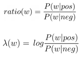
For each word of the table above, we could compute a “ratio” between the positive and negative probabilities. For example, the word “I” has a ratio of $0.115/0.083 = 1.385$.
If the ratio is 1, it means that the word is “neutral”. If is $> 1$ means that that word tends to be positive and $< 1$ means that the word tends to be negative.
We have to add a “ratio” in the Naive Bayes’ formula between the positive and negative tweets. Since in the example we had the same amount of positive/negative tweets, the ratio was 1.
\[\frac {P(Positive)} {P(Negative)} \prod_{i=1}^m \frac {P(w_i|Positive)} {P(w_i|Negative)}\]This is important for unbalanced data sets used for the training.
When computing these multiplications of probabilities, it is common to get really small numbers that can produce underflow when computing them (not being able to store the number). To avoid this situation, we apply the Log Likelihood.
Log Likelihood
To avoid the problem of underfitting, we can use the same expression but using logs.
\[log(\frac {P(Positive)} {P(Negative)} \prod_{i=1}^m \frac {P(w_i|Positive)} {P(w_i|Negative)}) = log(\frac {P(Positive)} {P(Negative)}) + \sum_{i=1}^m log(\frac {P(w_i|Positive)} {P(w_i|Negative)})\]This is true because of the logaritmic properrty that states that: $log({x}*{y}) = log(x) + log(y)$
If we apply the logarithm to the “ratio” just expressed above, you will usually see it represented as $\lambda$.
This mean that we can express the expression to do inference and detect if a tweet is positive by: $log(\frac {P(Positive)} {P(Negative)}) + log(\prod_{i=1}^m \frac {P(w_i|Positive)} {P(w_i|Negative)}) > 1 = log(\frac {P(Positive)} {P(Negative)}) + \sum_{i=1}^m \lambda(w_i) > 0$
Note that $log(\frac {P(Positive)} {P(Negative)})$ is known as the Log Prior
Wrapping it Up
To sum up, in order to build a Naïve Bayes classificator, we have to:
- Obtain a labeled dataset
- Preprocess the corpus (lowercasing, remove punctuation & stopwords, steaming and tokenize the sentence)
- Compute a frequency dictionary (the occurence of each word for each class)
- Get the \(P(w|Positive) \& P(w|Negative)\)
- Obtain the $\lambda(w)$ of each word doing: $log( \frac {P(w|Positive)} {P(w|Negative)})$
- Compute the log prior $log(\frac {P(Positive)} {P(Negative)})$
Now, if you would like to analyze the sentiment of a new text, you only need to obtain the $\lambda$ of each word that appears in the dictionary and summ all of them, plus the log prior.