Vector Space Models
Vector spaces models are algebraic models that can help us to better represent text. With vector space we can:
- Extract information and detect two senteces that are written different but have the same meaning
- Detect two sentences that are written almost the same but have differente meaning
- Detect corelation between words (summer —> hot, winter —>cold, etc.)
Building a Vector Space Model
There are different ways to start creating a vector space. The first step is to create a matrix. This matrix can be created using two different designs, word by word and word by document.
Word by Word
In the word by word design, each row and column corresponds to the same a word in the vocabulary. Then we can iterate word by word and count how many times a word appears next to each other from another word. The parameter \(K\) defines the “bandwith” that decides wether two words are next to each other or not. Here we have an example with \(K = 2\):
Corpus:
This is a hot summer
Last summer was hot and dry
We could built this matrix
| this | is | a | hot | last | was | … | |
|---|---|---|---|---|---|---|---|
| summer | 0 | 0 | 1 | 2 | 1 | 1 | … |
| … | … | … | … | … | … | … | … |
With this matrix we can represent each word as a vector.
Word by Document
In the word by document design, we apply the same concept but we map each word to a document type/class. The rows correspont to words and columns to documents/classes. Each number in the matrix is the number of times each word appears in a document or corpus classified with that class. Here we have another example. Imagine that we have 3 classes of documents: Sports, Economy and Science. Part of the matrix could look like this.
| Sports | Economy | Science | |
|---|---|---|---|
| points | 8000 | 4300 | 200 |
| cells | 100 | 200 | 7000 |
Now we can represent categories as vector too, for exaample Science is $v = [200, 7000]$
We could also plot this small example:

Euclidian Distance
Reusing the last example, we could compute the Eculidian distance between the “Economy” vector and the “Science” one. To do this we have to represent Economy and Science as two points:
Economy = (200, 4300)
Science = (7000, 200)
The Euclidian Distance between this two points is (Pitagoras theorem):
$d(B,A) = \sqrt{(B_1-A_1)^2+(B_2-A_2)^2}$
In the example: $\sqrt{(-6800)^2+(0)^2} = 6800$
If we have n dimensions, the expression is the same but considering each dimension:
$d(B,A) = \sqrt{(B_1-A_1)^2+(B_2-A_2)^2+… +(B_n-A_n)^2} = \sqrt{\sum_{i=1}^n(v_i-w_i)^2}$
This is also known as the Norm of the difference between the vectors $(\vec{v}-\vec{w})$:
$\sqrt{\sum_{i=1}^n(v_i-w_i)^2} = \parallel v - w \parallel$
In python, we can compute this with numpy with the “linalag” module, which provides linear algebra functions :
1
d = np.linalg.norm(v-w)
The Euclidean distance or similarity is not always the best way to compare documents that have different sizes because it does not take into account the differences in document length or size.
If two documents have different sizes, then the Euclidean distance between them can be biased towards the larger document, as it will have a greater number of dimensions in the feature space. This can lead to the smaller document being considered more dissimilar than it actually is.
Cosine Similarity
Cosine Similarity is another similarity score that can help us to avoid the problem that Euclidian Distance has with documents that have different sizes.
The Cosine Similarity searches the angle $\beta$ between two vectors. Before explaining how to obtain $\beta$, is important to remind the expressions of the:
Vector norm:
$\parallel \vec{v} \parallel = \sqrt{\sum_{i=1}^nv_i^2}$
In Python we can use
np.linalg.norm(v)
Dot product:
$\vec{v}·\vec{w}=\sum_{i=1}^nv_i · w_i$
The dot product can also be represented as
$\vec{v}·\vec{w}=\parallel \vec{v} \parallel \parallel \vec{w} \parallel cos(\beta)$
Hence:
$cos(\beta) = \frac {\vec{v}·\vec{w}} {\parallel \vec{v} \parallel \parallel \vec{w} \parallel}$
The closer to 1 is the result the more similar will be the vectors. The closer to 0, the more difference will be between two vectors.
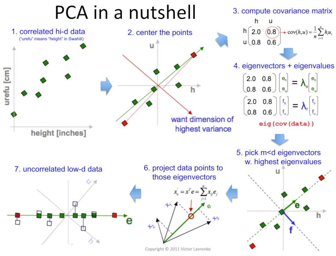
Principal Component Analysis
Now imagin that we are using the first technique to represent a word as a vector (word by word) but with a huge dataset. The vector would have a high dimensonality. To be more efficient, we want to reduce the noise and make use of low-dimensional representations that capture the most important information.
To achieve this, we will make use of the Principal Component Analysis (PCA). It is a dimensionality reduction method that simplifies the data by identifying the most important underlying features.
The goal of PCA is to identify the directions in the data that have the highest variance, and then project the data onto these directions. This is achieved by finding the eigenvectors and eigenvalues of the covariance matrix of the data. The eigenvectors correspond to the principal components, and the eigenvalues indicate how much of the variance in the data is captured by each component.
The eigenvectors represent the directions of highest variance in the data, and the corresponding eigenvalues indicate how much variance is captured in each direction. In other words, the larger the eigenvalue, the more important the corresponding eigenvector is in describing the data.
The steps that we have to follow in order to apply PCA are:
Data preprocessing: First, you need to preprocess your data to ensure that it is in the appropriate format for PCA. Specifically, you should center and scale your data so that each feature has zero mean and unit variance. You can do this by applying mean normalization:
$x_i = \frac {x_i - \mu_{x_i}} {\sigma_{x_i}}$
or de-meaning: $x_i = {x_i - \mu_{x_i}}$
Compute the covariance matrix: The covariance matrix measures the linear relationship between pairs of features in the data. You can compute the covariance matrix using the formula: $C = (1/n) * X^T * X$ where $n$ is the number of data points, $X$ is the data matrix, and $^T$ denotes the transpose of a matrix.
In Python we can use np.cov(X)
- Once we have the covariance matrix, we can apply a numerical linear algebra library or software package to perform the SVD (Single Value Decomposition) of the covariance matrix. The SVD of the covariance matrix will give you three matrices: U, Σ, and V. U and V are orthogonal matrices, while Σ is a diagonal matrix. The columns of U correspond to the eigenvectors of the covariance matrix, and the diagonal elements of Σ correspond to the square roots of the eigenvalues of the covariance matrix.
- To reduce the dimensionality of the data, you can select the first k columns of U and the first k rows and columns of Σ, where k is the desired number of dimensions. The resulting matrices can be multiplied to obtain a reduced-dimension representation of the data.