
Machine Translation
In this post we will learn how machines can translate text into different languages.
Imagine that we have all words in english represented as vectors and all words in french represented in vectors too. Each language will represent a vector space, so if we want to translate a word in english to french, we have to obtain the english word vector and transform it to the french vector space.
This transformation will be done using a transformation matrix.
Remember that if we multiply a vector with a matrix, we get a vector as result.
But, how do we obtain this transformation matrix?
Imagine that $X$ are the words in english, $R$ is the transformation matrix and $Y$ are the words in french.
$XR \approx Y$
If the first row in $X$ contains the vector of the word “hello”, the first row in $Y$ has to contain the vector of “bonjour”
$X$ and $Y$ doesn’t have to contain all words in each language, with a representative subset we can obtain R use it to traduce all the words.
We can start with a random $R$ and enhance it using gradient descent like we did in linear and logistic regression.
$Loss = | XR - F |^2_F$
repeat until it converges:
{
$g = \frac d {dR} Loss = \frac 2 m (X^T (XR-Y))$
$R = R - \alpha g$
}
$| XR - F |F$ is the Forbenius norm of $XR - F$. The Forbenious norm of A would be represented as: $|A|_F = \sqrt{\sum^m{i=1}\sum^n_{j=1} |a_{ij}|^2}$ (square root of the sum of the squares of all the entries in the matrix) Note that in the Loss function we do the square of the Forbenius norm so we cancel the square root.
Remember that $\alpha$ was the learning rate.
Once we have our transformation matrix, if we apply it to a english word, we may not get the exact vector for the word in french. To decide what word we should choose, we will use the K-nearest neighbors.
Locality Sensitive Hashing
Before talking about K-nearest neighbors, we need to define the Locality Sensitive Hashing, which is a technique used to efficiently approximate the similarity between two high-dimensional data points.
The idea is to hash data points into buckets (or groups) in such a way that similar points are more likely to be hashed into the same bucket than dissimilar points. This is achieved by defining a hash function that maps data points into a set of buckets, such that the probability of two similar points being hashed into the same bucket is higher than the probability of two dissimilar points being hashed into the same bucket.
A hash function is a mathematical function that takes in an input and produces a fixed-size output that represents the input data in a way that is more efficient to process or compare.
To do this, we will use vectors and “hyperplanes”. The hyperplanes are randomly generated during the construction of the hash function and are used to divide the space into smaller subspaces or partitions.
To hash a data point into a bucket, the hash function computes the dot product between the data point and a normal vector of a hyperplane. If the result of the dot product is positive, the data point is considered to be on one side of the hyperplane, and if the result is negative, it is on the other side. The hash function then uses the sign of the dot product to decide which of two subspaces the data point belongs to, and assigns it to the corresponding hash bucket. But… why?
Check this example in 2D. The green line represents a plane. P(4,4) is the normal vector of the plane (a vector perpendicular to that plane).
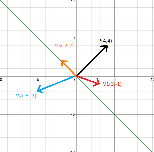
Now, lets pick he red vector V1(3,-1) and compute de dot product between P and V1:
$P \cdot V1 = 4 \cdot 3 + 4 \cdot -1 = 8$
Lets do the same with the other vectors: $P \cdot V2 = 4 \cdot -5 + 4 \cdot -2 = -28$
$P \cdot V3 = 4 \cdot -2 + 4 \cdot 2 = 0$
Note that when the vector is at one part of the plane, the result of the dot product with the normal vector is positive (V1 in the example), and if the vector is on the other side of the plane, the result is negative (V2 in the example). If the Vector is in the same plane (V3 in the example) the result will be 0.
Using this technique, we will be able to classify vectors into different buckets/groups
However, in real situations we will have more than one plane. For each vector we will need to compute the dot product with the normal vector of each plane. If we obtain a positive value we can assign a 1 for that vector-plane relation, if it is a negative or zero, we can assign a 0. Once we have all values for each relation between the vector and all the planes, we can invent a hash function to compute a value that represents the bucket.
If another vector gets the same results for all planes, the hash function will give us the same value so both vectors will be classified in the same bucket.
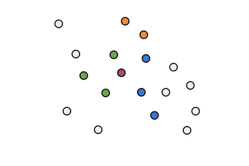
But, how do we know if the planes are correctly placed? We don’t. That’s why we will create multiple random planes and search for the other vectors that are in the same bucket for each iteration. We will provably get different results and discover more neighbors. In the example below, imagine that we are trying to search the k-nearest neighbors of the red dot that represents a vector. In the first iteration, the green points were in the same bucket. However, in the second interation with new planes, the blue points were in the same bucket, same with the third iteration and yellow points. This is how to find the Approximate nearest neighbors.
If we return to the original goal to translate a word, we can pick the nearest neighbor from all of them and assume that this is the translated word.